[사전학습] 6.3 회귀분석
회귀분석
단순회귀분석
한 개의 종속변수(Y)와 한 개의 독립변수(X) 사이의 관계를 분석하는 통계 기법
=> Y와 X간의 관계를 일차식(선형)에 대입하여, X의 변화에 따라 Y가 얼마나 변하는지를 예측할 때 사용
회귀분석 기본 과정
- 선형성 : 독리변수(X)와 종속변수(Y)는 선형관계이다.
- 독립성 : 종속변수 Y는 서로 독립이어야 한다. (한 관측 값이 다른 관측치에 의해 영향을 받으면 안됨)
- 등분산성 : 독립변수 X의 값에 관계없이 종속변수 Y의 분산은 일정하다.
- 정규성 : 독립변수 X의 고정된 어떤 값에 대하여 종속변수 Y는 정규분포를 따른다.
최소제곱법(OLS)
잔차의 제곱의 합을 최소화
결정계수($R^2$)
전체 제곱합(SST) = 회귀 제곱합(SSR) + 잔차 제곱합(SSE)
t 검정
단순회귀계수를 검정할 때, 개별회귀계수의 통계적 유의성은 t 검정으로 확인
다중회귀분석
단순회귀분석의 확장으로 독립변수가 두 개 이상인 회귀모형에 대한 분석
- 다중선형회귀모델 : $Y_i = \beta_0 + \beta_1X_{1i} + \beta_2X_{2i} + \cdots + \beta_kX_{ki} + e_i$ (단, $i = 1, 2, \cdots, n$)
- 단순회귀와의 차이점 : 단일 개의 독립변수가 아닌 여러 개의 독립변수를 사용
- 다중공선성 :
- 다중선형회귀분석 : 각 독립변수 간 독립성 가정
- 다중공선성 : 독립변수 간 상관성 존재를 의미 -> 독립성 x
=> 여러 개의 독립변수가 존재할 때 종속변수의 영향을 주는 독립변수를 찾는 것이 중요하며 최적의 변수 선택의 필요
이차회귀모델
비선형성을 고려한 이차회귀분석
다항회귀모델
3차, 4차 등과 같은 다항회귀모델이 있음
- 2차 이상의 회귀 모형
- 변수 간 상호작용 가능(Interaction)
- 장점 : 비선형적 추세를 고려할 수 있음
데이터에 따라서 Log나 차분을 통한 선형화로 계산을 용이하게 할 수 있음
실습
1
2
3
4
5
6
7
8
9
import numpy as np
import pandas as pd
import matplotlib.pyplot as plt
import seaborn as sns

from scipy import stats
import statsmodels.api as sm    # 회귀분석

from sklearn.datasets import load_boston
1
2
3
4
5
6
boston = load_boston()

X = boston.data
boston_df = pd.DataFrame(X, columns=boston.feature_names)
boston_df['MEDV'] = boston.target
boston_df
| CRIM | ZN | INDUS | CHAS | NOX | RM | AGE | DIS | RAD | TAX | PTRATIO | B | LSTAT | MEDV | |
|---|---|---|---|---|---|---|---|---|---|---|---|---|---|---|
| 0 | 0.00632 | 18.0 | 2.31 | 0.0 | 0.538 | 6.575 | 65.2 | 4.0900 | 1.0 | 296.0 | 15.3 | 396.90 | 4.98 | 24.0 |
| 1 | 0.02731 | 0.0 | 7.07 | 0.0 | 0.469 | 6.421 | 78.9 | 4.9671 | 2.0 | 242.0 | 17.8 | 396.90 | 9.14 | 21.6 |
| 2 | 0.02729 | 0.0 | 7.07 | 0.0 | 0.469 | 7.185 | 61.1 | 4.9671 | 2.0 | 242.0 | 17.8 | 392.83 | 4.03 | 34.7 |
| 3 | 0.03237 | 0.0 | 2.18 | 0.0 | 0.458 | 6.998 | 45.8 | 6.0622 | 3.0 | 222.0 | 18.7 | 394.63 | 2.94 | 33.4 |
| 4 | 0.06905 | 0.0 | 2.18 | 0.0 | 0.458 | 7.147 | 54.2 | 6.0622 | 3.0 | 222.0 | 18.7 | 396.90 | 5.33 | 36.2 |
| ... | ... | ... | ... | ... | ... | ... | ... | ... | ... | ... | ... | ... | ... | ... |
| 501 | 0.06263 | 0.0 | 11.93 | 0.0 | 0.573 | 6.593 | 69.1 | 2.4786 | 1.0 | 273.0 | 21.0 | 391.99 | 9.67 | 22.4 |
| 502 | 0.04527 | 0.0 | 11.93 | 0.0 | 0.573 | 6.120 | 76.7 | 2.2875 | 1.0 | 273.0 | 21.0 | 396.90 | 9.08 | 20.6 |
| 503 | 0.06076 | 0.0 | 11.93 | 0.0 | 0.573 | 6.976 | 91.0 | 2.1675 | 1.0 | 273.0 | 21.0 | 396.90 | 5.64 | 23.9 |
| 504 | 0.10959 | 0.0 | 11.93 | 0.0 | 0.573 | 6.794 | 89.3 | 2.3889 | 1.0 | 273.0 | 21.0 | 393.45 | 6.48 | 22.0 |
| 505 | 0.04741 | 0.0 | 11.93 | 0.0 | 0.573 | 6.030 | 80.8 | 2.5050 | 1.0 | 273.0 | 21.0 | 396.90 | 7.88 | 11.9 |
506 rows × 14 columns
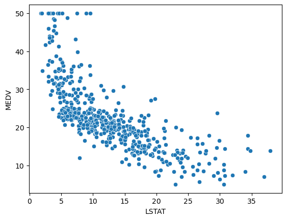
단순 회귀
산점도로 변수간 관계 파악
1
2
sns.scatterplot(x=boston_df['LSTAT'], y=boston_df['MEDV'])
plt.show()
1
2
MEDV = boston_df['MEDV'].values
LSTAT = boston_df['LSTAT'].values
독립변수에 상수항 결합
1
2
LSTAT = sm.add_constant(LSTAT)
LSTAT
1
2
3
4
5
6
7
array([[1.  , 4.98],
       [1.  , 9.14],
       [1.  , 4.03],
       ...,
       [1.  , 5.64],
       [1.  , 6.48],
       [1.  , 7.88]])
단순 선형 회귀 분석
1
2
linear_mod = sm.OLS(MEDV, LSTAT)
linear_mod
1
<statsmodels.regression.linear_model.OLS at 0x1730d52b408>
1
2
linear_result = linear_mod.fit()
linear_result
1
<statsmodels.regression.linear_model.RegressionResultsWrapper at 0x1730b014708>
1
print(linear_result.summary())
1
2
3
4
5
6
7
8
9
10
11
12
13
14
15
16
17
18
19
20
21
22
23
24
25
                            OLS Regression Results
==============================================================================
Dep. Variable:                      y   R-squared:                       0.544
Model:                            OLS   Adj. R-squared:                  0.543
Method:                 Least Squares   F-statistic:                     601.6
Date:                Tue, 31 Jan 2023   Prob (F-statistic):           5.08e-88
Time:                        09:11:05   Log-Likelihood:                -1641.5
No. Observations:                 506   AIC:                             3287.
Df Residuals:                     504   BIC:                             3295.
Df Model:                           1
Covariance Type:            nonrobust
==============================================================================
                 coef    std err          t      P>|t|      [0.025      0.975]
------------------------------------------------------------------------------
const         34.5538      0.563     61.415      0.000      33.448      35.659
x1            -0.9500      0.039    -24.528      0.000      -1.026      -0.874
==============================================================================
Omnibus:                      137.043   Durbin-Watson:                   0.892
Prob(Omnibus):                  0.000   Jarque-Bera (JB):              291.373
Skew:                           1.453   Prob(JB):                     5.36e-64
Kurtosis:                       5.319   Cond. No.                         29.7
==============================================================================

Notes:
[1] Standard Errors assume that the covariance matrix of the errors is correctly specified.
1
np.sqrt(linear_result.fvalue)
1
24.527899851187733
1
2
linear_mod = sm.OLS.from_formula("MEDV ~ LSTAT", data=boston_df)
linear_result = linear_mod.fit()
1
print(linear_result.summary())
1
2
3
4
5
6
7
8
9
10
11
12
13
14
15
16
17
18
19
20
21
22
23
24
25
                            OLS Regression Results
==============================================================================
Dep. Variable:                   MEDV   R-squared:                       0.544
Model:                            OLS   Adj. R-squared:                  0.543
Method:                 Least Squares   F-statistic:                     601.6
Date:                Tue, 31 Jan 2023   Prob (F-statistic):           5.08e-88
Time:                        09:14:28   Log-Likelihood:                -1641.5
No. Observations:                 506   AIC:                             3287.
Df Residuals:                     504   BIC:                             3295.
Df Model:                           1
Covariance Type:            nonrobust
==============================================================================
                 coef    std err          t      P>|t|      [0.025      0.975]
------------------------------------------------------------------------------
Intercept     34.5538      0.563     61.415      0.000      33.448      35.659
LSTAT         -0.9500      0.039    -24.528      0.000      -1.026      -0.874
==============================================================================
Omnibus:                      137.043   Durbin-Watson:                   0.892
Prob(Omnibus):                  0.000   Jarque-Bera (JB):              291.373
Skew:                           1.453   Prob(JB):                     5.36e-64
Kurtosis:                       5.319   Cond. No.                         29.7
==============================================================================

Notes:
[1] Standard Errors assume that the covariance matrix of the errors is correctly specified.
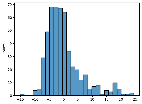
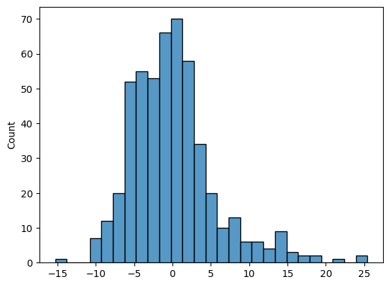
잔차 확인
1
2
sns.histplot(linear_result.resid)
plt.show()
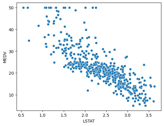
선형화를 통한 회귀분석
상관관계 및 분포 확인
1
2
sns.pairplot(boston_df[['LSTAT', 'MEDV']])
plt.show()

1
2
sns.scatterplot(x=np.log(boston_df['LSTAT']), y=boston_df['MEDV'])
plt.show()
회귀 분석
1
2
log_linear_mod = sm.OLS.from_formula("MEDV ~ np.log(LSTAT)", data=boston_df)
log_linear_result = log_linear_mod.fit()
1
print(log_linear_result.summary())
1
2
3
4
5
6
7
8
9
10
11
12
13
14
15
16
17
18
19
20
21
22
23
24
25
                            OLS Regression Results
==============================================================================
Dep. Variable:                   MEDV   R-squared:                       0.665
Model:                            OLS   Adj. R-squared:                  0.664
Method:                 Least Squares   F-statistic:                     1000.
Date:                Tue, 31 Jan 2023   Prob (F-statistic):          9.28e-122
Time:                        13:43:33   Log-Likelihood:                -1563.6
No. Observations:                 506   AIC:                             3131.
Df Residuals:                     504   BIC:                             3140.
Df Model:                           1
Covariance Type:            nonrobust
=================================================================================
                    coef    std err          t      P>|t|      [0.025      0.975]
---------------------------------------------------------------------------------
Intercept        52.1248      0.965     54.004      0.000      50.228      54.021
np.log(LSTAT)   -12.4810      0.395    -31.627      0.000     -13.256     -11.706
==============================================================================
Omnibus:                      126.181   Durbin-Watson:                   0.918
Prob(Omnibus):                  0.000   Jarque-Bera (JB):              323.855
Skew:                           1.237   Prob(JB):                     4.74e-71
Kurtosis:                       6.039   Cond. No.                         11.5
==============================================================================

Notes:
[1] Standard Errors assume that the covariance matrix of the errors is correctly specified.
2차 회귀 분석 (Quadrratic Regression Model)
1
2
sns.pairplot(boston_df[['LSTAT', 'MEDV']])
plt.show()
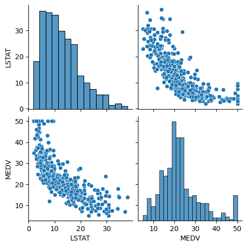
- 두 변수간 커브 모양의 관계형성 확인 -> 이를 고려하기 위해
LSTAT변수의 2차항을 추가
1
2
3
quadratic_mod = sm.OLS.from_formula("MEDV ~ LSTAT + I(LSTAT ** 2)", data=boston_df)
quadratic_result = quadratic_mod.fit()
print(quadratic_result.summary())
1
2
3
4
5
6
7
8
9
10
11
12
13
14
15
16
17
18
19
20
21
22
23
24
25
26
27
28
                            OLS Regression Results
==============================================================================
Dep. Variable:                   MEDV   R-squared:                       0.641
Model:                            OLS   Adj. R-squared:                  0.639
Method:                 Least Squares   F-statistic:                     448.5
Date:                Tue, 31 Jan 2023   Prob (F-statistic):          1.56e-112
Time:                        13:47:32   Log-Likelihood:                -1581.3
No. Observations:                 506   AIC:                             3169.
Df Residuals:                     503   BIC:                             3181.
Df Model:                           2
Covariance Type:            nonrobust
=================================================================================
                    coef    std err          t      P>|t|      [0.025      0.975]
---------------------------------------------------------------------------------
Intercept        42.8620      0.872     49.149      0.000      41.149      44.575
LSTAT            -2.3328      0.124    -18.843      0.000      -2.576      -2.090
I(LSTAT ** 2)     0.0435      0.004     11.628      0.000       0.036       0.051
==============================================================================
Omnibus:                      107.006   Durbin-Watson:                   0.921
Prob(Omnibus):                  0.000   Jarque-Bera (JB):              228.388
Skew:                           1.128   Prob(JB):                     2.55e-50
Kurtosis:                       5.397   Cond. No.                     1.13e+03
==============================================================================

Notes:
[1] Standard Errors assume that the covariance matrix of the errors is correctly specified.
[2] The condition number is large, 1.13e+03. This might indicate that there are
strong multicollinearity or other numerical problems.
잔차 확인
1
2
sns.histplot(quadratic_result.resid)
plt.show()
3개 모델 결과 비교 (선형 vs Log-Linear vs 2차 회귀)
1
2
3
print("Linear Model :", np.round(linear_result.rsquared, 2))
print("Log-Linear Model :", np.round(log_linear_result.rsquared, 2))
print("Quadratic Model :", np.round(quadratic_result.rsquared, 2))
1
2
3
Linear Model : 0.54
Log-Linear Model : 0.66
Quadratic Model : 0.64
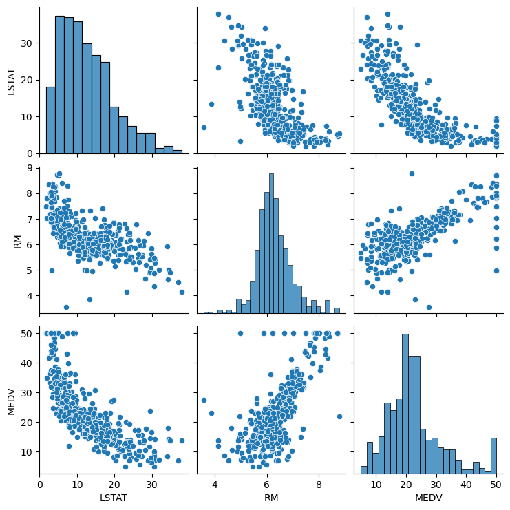
다중 회귀 (Multiple Regression)
1
2
sns.pairplot(boston_df[['LSTAT', 'RM', 'MEDV']])
plt.show()
1
2
3
4
multi_model = sm.OLS.from_formula("MEDV ~ RM + LSTAT + I(LSTAT ** 2)", data=boston_df)
multi_result = multi_model.fit()

print(multi_result.summary())
1
2
3
4
5
6
7
8
9
10
11
12
13
14
15
16
17
18
19
20
21
22
23
24
25
26
27
28
29
                            OLS Regression Results
==============================================================================
Dep. Variable:                   MEDV   R-squared:                       0.703
Model:                            OLS   Adj. R-squared:                  0.701
Method:                 Least Squares   F-statistic:                     396.2
Date:                Tue, 31 Jan 2023   Prob (F-statistic):          6.50e-132
Time:                        13:51:30   Log-Likelihood:                -1533.0
No. Observations:                 506   AIC:                             3074.
Df Residuals:                     502   BIC:                             3091.
Df Model:                           3
Covariance Type:            nonrobust
=================================================================================
                    coef    std err          t      P>|t|      [0.025      0.975]
---------------------------------------------------------------------------------
Intercept        11.6896      3.138      3.725      0.000       5.524      17.855
RM                4.2273      0.412     10.267      0.000       3.418       5.036
LSTAT            -1.8486      0.122    -15.136      0.000      -2.089      -1.609
I(LSTAT ** 2)     0.0363      0.003     10.443      0.000       0.030       0.043
==============================================================================
Omnibus:                      123.119   Durbin-Watson:                   0.848
Prob(Omnibus):                  0.000   Jarque-Bera (JB):              411.618
Skew:                           1.105   Prob(JB):                     4.15e-90
Kurtosis:                       6.826   Cond. No.                     4.49e+03
==============================================================================

Notes:
[1] Standard Errors assume that the covariance matrix of the errors is correctly specified.
[2] The condition number is large, 4.49e+03. This might indicate that there are
strong multicollinearity or other numerical problems.
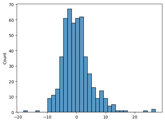
잔차 확인
1
2
sns.histplot(multi_result.resid)
plt.show()
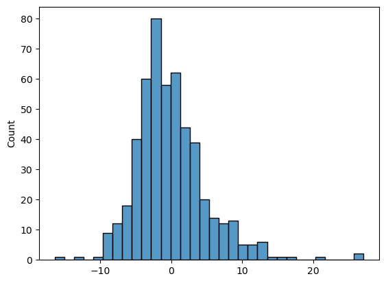
로그항 추가 (2차항 제거)
1
2
3
4
multi_model2 = sm.OLS.from_formula("MEDV ~ RM + np.log(LSTAT)", data=boston_df)
multi_result2 = multi_model2.fit()

print(multi_result2.summary())
1
2
3
4
5
6
7
8
9
10
11
12
13
14
15
16
17
18
19
20
21
22
23
24
25
26
                            OLS Regression Results
==============================================================================
Dep. Variable:                   MEDV   R-squared:                       0.707
Model:                            OLS   Adj. R-squared:                  0.706
Method:                 Least Squares   F-statistic:                     607.2
Date:                Tue, 31 Jan 2023   Prob (F-statistic):          7.40e-135
Time:                        13:52:56   Log-Likelihood:                -1529.6
No. Observations:                 506   AIC:                             3065.
Df Residuals:                     503   BIC:                             3078.
Df Model:                           2
Covariance Type:            nonrobust
=================================================================================
                    coef    std err          t      P>|t|      [0.025      0.975]
---------------------------------------------------------------------------------
Intercept        22.8865      3.552      6.443      0.000      15.908      29.865
RM                3.5977      0.423      8.512      0.000       2.767       4.428
np.log(LSTAT)    -9.6855      0.494    -19.597      0.000     -10.656      -8.714
==============================================================================
Omnibus:                      130.413   Durbin-Watson:                   0.850
Prob(Omnibus):                  0.000   Jarque-Bera (JB):              421.915
Skew:                           1.185   Prob(JB):                     2.41e-92
Kurtosis:                       6.794   Cond. No.                         111.
==============================================================================

Notes:
[1] Standard Errors assume that the covariance matrix of the errors is correctly specified.
잔차 확인
1
2
sns.histplot(multi_result2.resid)
plt.show()
성능 확인
1
2
print("Multiple Regression Model (2차항 포함) : {:.3f}".format(multi_result.rsquared))
print("Multiple Regression Model (로그 변환항 포함) : {:.3f}".format(multi_result2.rsquared))
1
2
Multiple Regression Model (2차항 포함) : 0.703
Multiple Regression Model (로그 변환항 포함) : 0.707
1
This post is licensed under CC BY 4.0 by the author.