[사전학습] 6.4 시계열 분석
시계열 분석
시계열 데이터
순차적인 시간의 흐름에 따라 기록된 데이터를 의미
Y = T + S + C + R 또는 Y + T X S X C X R
- 추세 (Trend) : 시간의 흐름에 따라 점진적이고 지속적인 변화
- 계절성(Seasonality) : 특정 주기에 따라 일정한 패턴을 갖는 변화
- 싸이클(Cycle) : 경제 또는 사회적 요인에 의한 변화(예: 경기 변동)이며, 일정 주기가 없고 장기적인 변화
- 잔차(Residuals) : 설명할 수 없는 변화
시계열 분석의 특징
현재 시점의 시계열 데이터를 분석하는데 이전 시간의 값이 현재에도 영향을 끼칠 것이라는 가정하에 회귀분석을 진행
시계계열 분석 vs 단순 회귀
| 시계열 분석 | 단순 회귀 |
|---|---|
| 자기 상관(Autocorrelation) 존재 | 자기 상관(Autocorrelation) 없음 |
| 대표적으로 자기회귀, 이동평균, 자기회귀누적이동평균, 벡터자기회귀 모델 등이 존재 | 독립변수와 종속변수는 서로 다른 변수일 경우가 많음 |
| 현재 시점에 가까운 데이터일 수록 서로 강한 관계를 맺는 경향 존재 | 선형 회귀로 시계열 데이터를 분석하려면 더 까다로운 가정 필요(선형성 가정이 필요) |
자기회귀 모델 (AR)
AR 모델은 시계열의 미대 값이 과거 값에 기반한다는 모델. 즉, 이전 값의 영향을 받는 것이 특징
이동평균 모델 (MA)
전체적인 편향성을 다루는 모델로, 설명변수가 최근 오차항으로만 구성되어 있는 것이 특징
이전 시점의 값에 기반하는 것이 아닌 이전 시점의 예측 오차에 가중치를 두어 미래의 값을 예측
ARIMA 모델
AR과 MA를 동시에 고려하고, 누적(I)으로 추세까지 고려한 모델로, ‘자기회귀 누적 이동평균 모델’이라고도 불림
ARIMA(p, d, q) = AR(p) + I(d) + MA(q)
- AR이나 MA 모델 혼자로는 역동성을 설명하기엔 부족한 경우가 있음 -> ARMA 모델로 결합
- 정상성 만족을 위해 차분이 가미되면서 ARIMA가 됨
정상성
정상성을 나타내는 시계열은 관측치가 시간과 무관해야 함 (즉 시간에 상관없이 일정한 평균과 분산을 갖고 있어야 함)
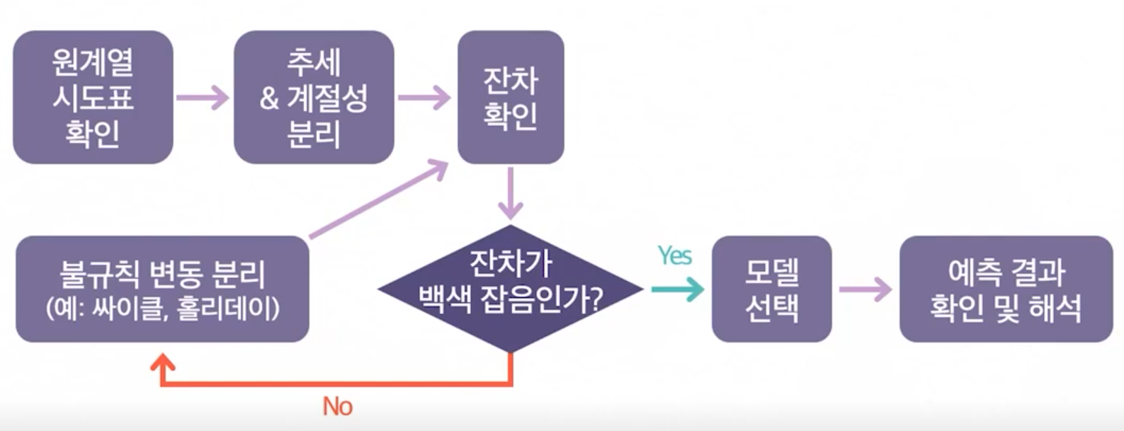
시계열 분석 순서
실습
1
2
3
4
5
6
7
8
9
10
import pandas as pd
import numpy as np
import matplotlib.pyplot as plt

import statsmodels.api as sm
from statsmodels.tsa.stattools import adfuller  # ADF는 정상성 검정을 위해 사용
from statsmodels.tsa.seasonal import seasonal_decompose # 시계열 요소 분해
from statsmodels.tsa.arima.model import ARIMA # ARIMA 모델, SARIMA 모델

import pmdarima as pm # auto arima
정상성 vs 비정상성
정상성
정상성을 띄는 시계열은 해당 시계열이 관측된 시간과 무관 (즉, 시간에 따라 상승하거나 주기적인 변화가 있는 추세나 계절성이 없음)
- 특징
- 정상 시계열은 평균이 일정
- 분산이 시점에 의존하지 않음
- 공분산은 시점에 의존하지 않음 (시차에는 의존)
- 정상성을 띄는 시계열은 장기적으로 예측 불가능한 시계열 (e.g. 백색잡음 white noise가 대표적인 예)
비정상성
시간에 영향을 받는 시계열 (추세나 계절성이 있는 것이 대표적인 특징)
- 특징
- 시간의 흐름에 따라 시계열의 평균 수준이 다름
- 시간의 흐름에 따라 추세를 가짐 (우상향, 우하향 추세 등)
- 시간의 흐름에 따라 계절성이 있음
- 시간의 흐름에 따라 시계열의 분산이 증가하거나 감소함
- 비정상 시계열 예제) 여름에 아이스크림 판매량이 높으며 겨울에 판매량이 낮다(계절성)
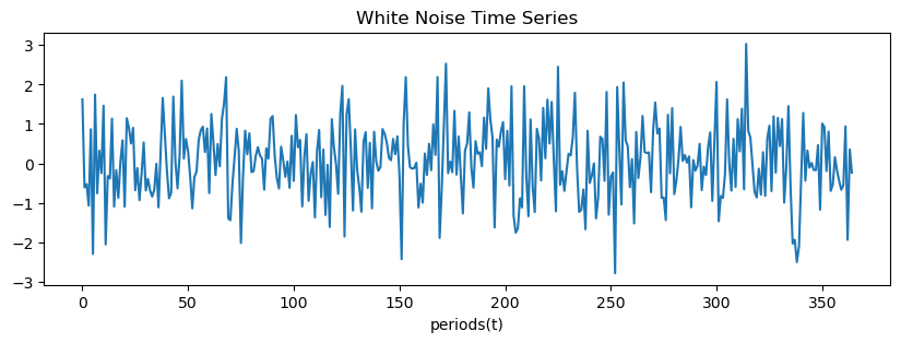
정상 시계열 - 백색잡음 (white noise)
1
2
3
np.random.seed(1)

x = np.random.randn(365)
원계열 시도표 (Time Plot)
1
2
3
4
5
6
plt.figure(figsize=(10, 3))

plt.plot(np.arange(365), x)
plt.title('White Noise Time Series')
plt.xlabel('periods(t)')
plt.show()
Augmented Dickey Fuller Test 단위근 검정 (ADF test)
- $H_0$ : 정상성이 있는 시계열이 아님 (단위근)
- $H_1$ : 정상성이 있는 시계열
- 귀무가설을 기각해야 정상성이 있는 시계열
1
2
result = adfuller(x)
result
1
2
3
4
5
6
7
8
(-19.77252320210403,
 0.0,
 0,
 364,
 {'1%': -3.4484434475193777,
  '5%': -2.869513170510808,
  '10%': -2.571017574266393},
 952.9340604979548)
1
2
3
4
5
print('ADF stat : {:.4f}'.format(result[0]))
print('p-value : {:.4f}'.format(result[1]))
print('Critical Values : ')
for key, value in result[4].items():
    print('\t{} : {:.4f}'.format(key, value))
1
2
3
4
5
6
ADF stat : -19.7725
p-value : 0.0000
Critical Values :
	1% : -3.4484
	5% : -2.8695
	10% : -2.5710
ACF와 PACF
1
2
3
4
5
6
fig, axes = plt.subplots(1, 2, figsize=(15, 4))

fig = sm.graphics.tsa.plot_acf(x, lags=40, ax=axes[0])
fig = sm.graphics.tsa.plot_pacf(x, lags=40, ax=axes[1])
fig.suptitle('ACF and PACF Graph of White Noise', y=1.05)
plt.show()
1
2
c:\Users\zxwlg\miniconda3\envs\dx_env\lib\site-packages\statsmodels\graphics\tsaplots.py:353: FutureWarning: The default method 'yw' can produce PACF values outside of the [-1,1] interval. After 0.13, the default will change tounadjusted Yule-Walker ('ywm'). You can use this method now by setting method='ywm'.
  FutureWarning,
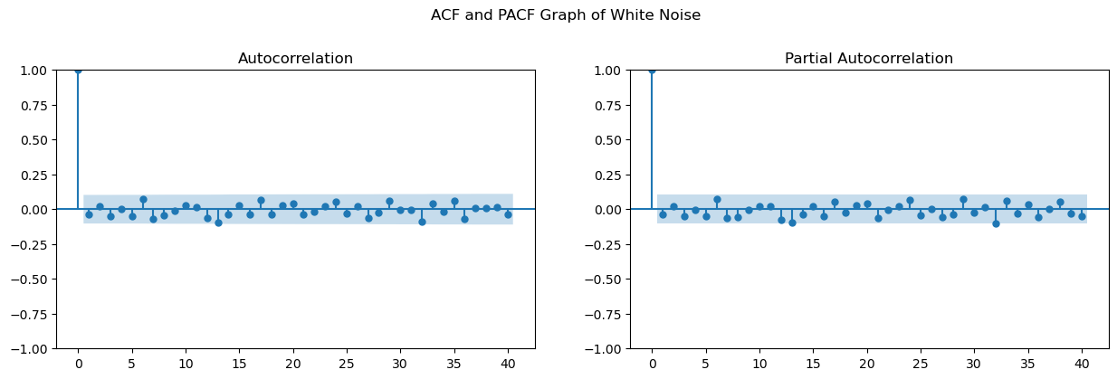
자기상관 및 편자기상관 없음 -> 정상성
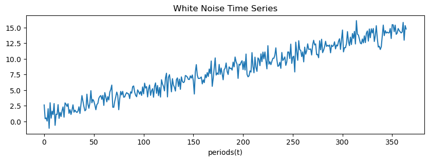
비정상성 시계열 (추세 존재)
1
2
trend = np.linspace(1, 15, 365) # 추세 생성
x_w_trend = x + trend # 백색잡음 x에 추세 추가
원계열 시도표 (Time Plot)
1
2
3
4
5
6
plt.figure(figsize=(10, 3))

plt.plot(np.arange(365), x_w_trend)
plt.title('White Noise Time Series')
plt.xlabel('periods(t)')
plt.show()
Augmented Dickey Fuller Test 단위근 검정 (ADF test)
- $H_0$ : 정상성이 있는 시계열이 아님 (단위근)
- $H_1$ : 정상성이 있는 시계열
- 귀무가설을 기각해야 정상성이 있는 시계열
1
2
3
4
5
6
result = adfuller(x_w_trend)
print('ADF stat : {:.4f}'.format(result[0]))
print('p-value : {:.4f}'.format(result[1]))
print('Critical Values : ')
for key, value in result[4].items():
    print('\t{} : {:.4f}'.format(key, value))
1
2
3
4
5
6
ADF stat : -0.7079
p-value : 0.8447
Critical Values :
	1% : -3.4493
	5% : -2.8699
	10% : -2.5712
결론 : 귀무가설 기각 실패 -> 정상성 만족 x
ACF와 PACF
1
2
3
4
5
6
fig, axes = plt.subplots(1, 2, figsize=(15, 4))

fig = sm.graphics.tsa.plot_acf(x_w_trend, lags=40, ax=axes[0])
fig = sm.graphics.tsa.plot_pacf(x_w_trend, lags=40, ax=axes[1])
fig.suptitle('ACF and PACF Graph of White Noise', y=1.05)
plt.show()
1
2
c:\Users\zxwlg\miniconda3\envs\dx_env\lib\site-packages\statsmodels\graphics\tsaplots.py:353: FutureWarning: The default method 'yw' can produce PACF values outside of the [-1,1] interval. After 0.13, the default will change tounadjusted Yule-Walker ('ywm'). You can use this method now by setting method='ywm'.
  FutureWarning,
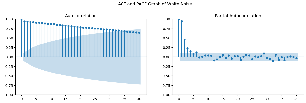
자기상관(Autocorrelation)은 시간이 흐를수록 줄어들고 있음 (파란 음영 부분 안으로 들어옴) & 편자기상관(Partial Autocorrelation)은 시차 5번째부터 파란 음영부분으로 들어왔음
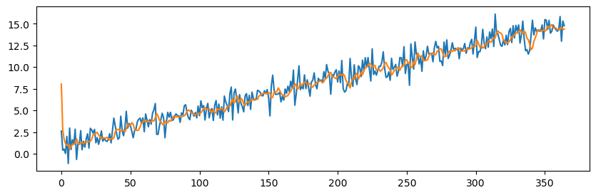
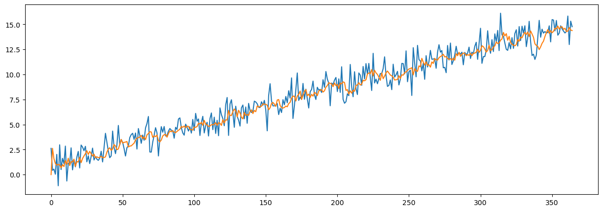
ARIMA – AR(5)
1
arima_mod = ARIMA(x_w_trend, order=(5, 0, 0)) # AR order만 5, 따라서 AR(5) 모델임
1
result = arima_mod.fit()
1
2
3
4
5
plt.figure(figsize=(10, 3))

plt.plot(np.arange(365), x_w_trend)
plt.plot(np.arange(365), result.fittedvalues)
plt.show()
1
print(result.summary())
1
2
3
4
5
6
7
8
9
10
11
12
13
14
15
16
17
18
19
20
21
22
23
24
25
26
27
28
                               SARIMAX Results
==============================================================================
Dep. Variable:                      y   No. Observations:                  365
Model:                 ARIMA(5, 0, 0)   Log Likelihood                -545.109
Date:                Tue, 31 Jan 2023   AIC                           1104.217
Time:                        17:54:46   BIC                           1131.516
Sample:                             0   HQIC                          1115.066
                                - 365
Covariance Type:                  opg
==============================================================================
                 coef    std err          z      P>|z|      [0.025      0.975]
------------------------------------------------------------------------------
const          8.0428      5.053      1.592      0.111      -1.861      17.947
ar.L1          0.1981      0.048      4.106      0.000       0.104       0.293
ar.L2          0.2489      0.052      4.796      0.000       0.147       0.351
ar.L3          0.1680      0.055      3.050      0.002       0.060       0.276
ar.L4          0.2175      0.049      4.423      0.000       0.121       0.314
ar.L5          0.1613      0.051      3.136      0.002       0.060       0.262
sigma2         1.1475      0.084     13.623      0.000       0.982       1.313
===================================================================================
Ljung-Box (L1) (Q):                   0.54   Jarque-Bera (JB):                 0.20
Prob(Q):                              0.46   Prob(JB):                         0.90
Heteroskedasticity (H):               1.28   Skew:                             0.05
Prob(H) (two-sided):                  0.17   Kurtosis:                         3.06
===================================================================================

Warnings:
[1] Covariance matrix calculated using the outer product of gradients (complex-step).
1
print('mean absolute error : {}'.format(result.mae))
1
mean absolute error : 0.8551272105200026
1
2
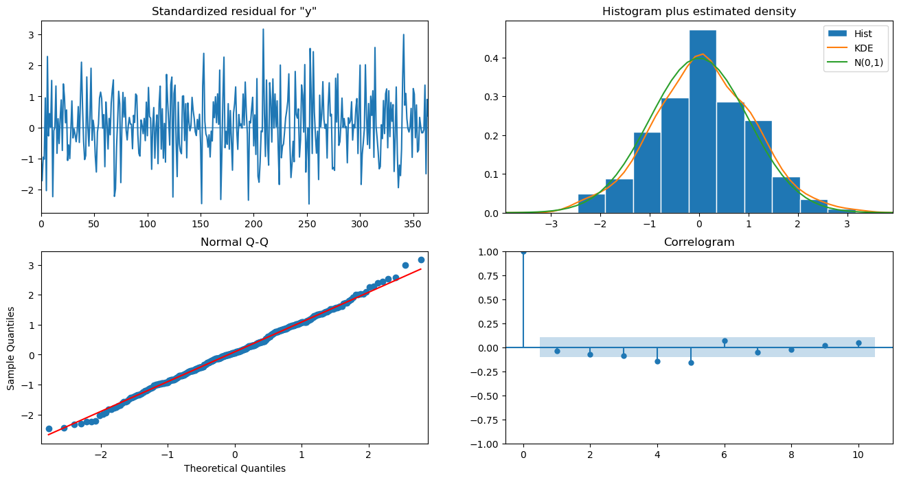
result.plot_diagnostics(figsize=(16, 8))
plt.show()
ARIMA – I(1)
1
2
arima_mod2 = ARIMA(x_w_trend, order=(0, 1, 0))
result = arima_mod2.fit()
1
2
3
4
5
plt.figure(figsize=(15, 5))

plt.plot(np.arange(365), x_w_trend)
plt.plot(np.arange(365), result.fittedvalues)
plt.show()
1
2
i_1 = np.sum(np.abs(np.abs(x_w_trend - result.fittedvalues)))
i_1
1
398.3766694444225
1
print(result.summary())
1
2
3
4
5
6
7
8
9
10
11
12
13
14
15
16
17
18
19
20
21
22
                               SARIMAX Results
==============================================================================
Dep. Variable:                      y   No. Observations:                  365
Model:                 ARIMA(0, 1, 0)   Log Likelihood                -634.642
Date:                Tue, 31 Jan 2023   AIC                           1271.284
Time:                        17:59:25   BIC                           1275.181
Sample:                             0   HQIC                          1272.833
                                - 365
Covariance Type:                  opg
==============================================================================
                 coef    std err          z      P>|z|      [0.025      0.975]
------------------------------------------------------------------------------
sigma2         1.9139      0.130     14.755      0.000       1.660       2.168
===================================================================================
Ljung-Box (L1) (Q):                 100.83   Jarque-Bera (JB):                 2.43
Prob(Q):                              0.00   Prob(JB):                         0.30
Heteroskedasticity (H):               1.21   Skew:                             0.05
Prob(H) (two-sided):                  0.29   Kurtosis:                         3.39
===================================================================================

Warnings:
[1] Covariance matrix calculated using the outer product of gradients (complex-step).
1
print('mean absolute error : {}'.format(result.mae))
1
mean absolute error : 1.091442929984719
1
2
3
4
from sklearn.metrics import mean_absolute_error

mae = mean_absolute_error(x_w_trend, result.fittedvalues)
print('mean absolute error : {}'.format(mae))
1
mean absolute error : 1.091442929984719
PM
1
2
3
4
5
6
7
8
9
10
11
pm.arima.auto_arima(
    x_w_trend,
    d=1,
    start_p=0,
    max_p=5,
    start_q=0,
    max_q=5,
    seasonal=False,
    step=True,
    trace=True
)
1
2
3
4
5
6
7
8
9
10
11
12
13
14
15
16
17
18
19
20
21
22
23
24
Performing stepwise search to minimize aic
 ARIMA(0,1,0)(0,0,0)[0] intercept   : AIC=1273.072, Time=0.01 sec
 ARIMA(1,1,0)(0,0,0)[0] intercept   : AIC=1157.411, Time=0.03 sec
 ARIMA(0,1,1)(0,0,0)[0] intercept   : AIC=inf, Time=0.13 sec
 ARIMA(0,1,0)(0,0,0)[0]             : AIC=1271.284, Time=0.01 sec
 ARIMA(2,1,0)(0,0,0)[0] intercept   : AIC=1125.228, Time=0.03 sec
 ARIMA(3,1,0)(0,0,0)[0] intercept   : AIC=1101.074, Time=0.06 sec
 ARIMA(4,1,0)(0,0,0)[0] intercept   : AIC=1092.347, Time=0.05 sec
 ARIMA(5,1,0)(0,0,0)[0] intercept   : AIC=1071.004, Time=0.09 sec
 ARIMA(5,1,1)(0,0,0)[0] intercept   : AIC=inf, Time=0.47 sec
 ARIMA(4,1,1)(0,0,0)[0] intercept   : AIC=inf, Time=0.35 sec
 ARIMA(5,1,0)(0,0,0)[0]             : AIC=1075.303, Time=0.05 sec

Best model:  ARIMA(5,1,0)(0,0,0)[0] intercept
Total fit time: 1.271 seconds


ARIMA(maxiter=50, method='lbfgs', order=(5, 1, 0), out_of_sample_size=0,
      scoring='mse', scoring_args={}, seasonal_order=(0, 0, 0, 0),
      start_params=None, suppress_warnings=True, trend=None,
      with_intercept=True)
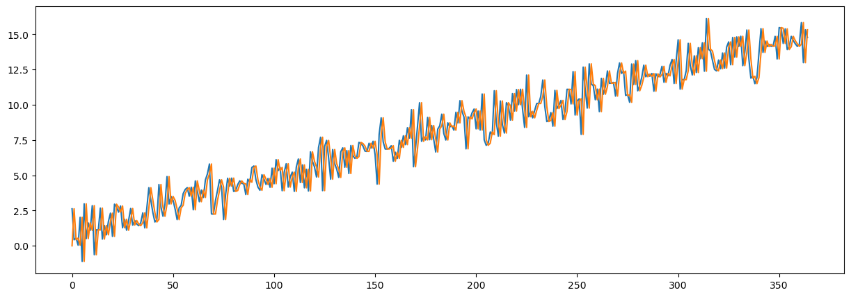
1
2
3
arima_mod3 = ARIMA(x_w_trend, order=(5, 1, 0))
result = arima_mod3.fit()
print(result.summary())
1
2
3
4
5
6
7
8
9
10
11
12
13
14
15
16
17
18
19
20
21
22
23
24
25
26
27
                               SARIMAX Results
==============================================================================
Dep. Variable:                      y   No. Observations:                  365
Model:                 ARIMA(5, 1, 0)   Log Likelihood                -531.651
Date:                Tue, 31 Jan 2023   AIC                           1075.303
Time:                        18:02:31   BIC                           1098.686
Sample:                             0   HQIC                          1084.596
                                - 365
Covariance Type:                  opg
==============================================================================
                 coef    std err          z      P>|z|      [0.025      0.975]
------------------------------------------------------------------------------
ar.L1         -0.8423      0.047    -17.886      0.000      -0.935      -0.750
ar.L2         -0.6425      0.069     -9.352      0.000      -0.777      -0.508
ar.L3         -0.5129      0.067     -7.630      0.000      -0.645      -0.381
ar.L4         -0.3512      0.065     -5.380      0.000      -0.479      -0.223
ar.L5         -0.2386      0.054     -4.416      0.000      -0.345      -0.133
sigma2         1.0835      0.083     13.035      0.000       0.921       1.246
===================================================================================
Ljung-Box (L1) (Q):                   0.22   Jarque-Bera (JB):                 0.08
Prob(Q):                              0.64   Prob(JB):                         0.96
Heteroskedasticity (H):               1.34   Skew:                            -0.02
Prob(H) (two-sided):                  0.11   Kurtosis:                         2.93
===================================================================================

Warnings:
[1] Covariance matrix calculated using the outer product of gradients (complex-step).
1
2
3
4
5
plt.figure(figsize=(15, 5))

plt.plot(np.arange(365), x_w_trend)
plt.plot(np.arange(365), result.fittedvalues)
plt.show()
1
print('mean absolute error : {}'.format(result.mae))
1
mean absolute error : 0.8300001373295226
시계열 성분 분해 (Time Series Decomposition)
샘플 데이터 필요
1
2
df = pd.read_csv('./data/latte_ice_cream.csv')
df
1
2
df['time'] = pd.to_datetime(df['year'].astype(str) + '-' + df['month'].astype(str) + '-' + df['date'].astype(str))
df
1
2
df = df.set_index('time', drop=True)
df
1
2
ts = df['sales_amount']
ts
시도표 (Time Plot)
1
2
ts.plot(figsize=(10, 3))
plt.show()
시도표를 보며 생각해볼 점.
1
2
3
4
5
6
fig, axes = plt.subplots(1, 2, figsize=(15, 4))

fig = sm.graphics.tsa.plot_acf(ts, lags=40, ax=axes[0])
fig = sm.graphics.tsa.plot_pacf(ts, lags=40, ax=axes[1])

plt.show()
생각해볼점 : 자기상관의 패턴은 어떠한가? 또한, 편 자기상관의 패턴은 어떠한가?
계절성 분해(seasonal_decompose)
1
2
3
4
decomp = seasonal_decompose(ts, model='additive', period=12)

fig = decomp.plot()
fig.set_size_inches((12, 8))
분해 후 남은 잔차(Resid)를 살펴보자. 시간의 흐름에 따라 동일한가 (homoskedastic)? 증가하는가/감소하는가 (heteroskedastic)?
1
2
3
4
decomp = seasonal_decompose(ts, model='multiplicative', period=12)

fig = decomp.plot()
fig.set_size_inches((12, 8))
분해 후 남은 잔차(Resid)를 살펴보자. 시간의 흐름에 따라 동일한가 (homoskedastic)? 증가하는가/감소하는가 (heteroskedastic)?
SARIMAX : ARIMA + 계절성 (S) = SARIMA
1
s_mod = sm.tsa.statespace.SARIMAX(ts, order=(1, 1, 0), seasonal_order=(1, 1, 0, 12))
1
2
result = s_mod.fit()
print(result.summary())
1
2
3
4
plt.figure(figsize=(10, 3))
plt.plot(ts)
plt.plot(result.fittedvalues, color='r')
plt.show()
1
2
3
4
5
6
7
8
9
10
11
12
13
pm.arima.auto_arima(
    ts,
    d=1,
    start_p=0,
    max_p=5,
    start_q=0,
    max_q=5,
    D=1,
    m=12,
    seasonal=True,
    step=True,
    trace=True
)
1
s_mod = sm.tsa.statespace.SARIMAX(ts, order=(0, 1, 1), seasonal_order=(1, 1, 2, 12))
1
2
result = s_mod.fit()
print(result.summary())
1
2
3
4
plt.figure(figsize=(10, 3))
plt.plot(ts)
plt.plot(result.fittedvalues, color='r')
plt.show()